Sometimes, coding can feel like solving a complicated puzzle. Sometimes, that puzzle boils down to “spot the differences.” Visual Studio Code (VS Code) lets you elegantly compare the contents of two files in a few simple steps. This guide will show you how easy it is to compare two different files in VS Code. There will also be some other nifty features that could make coding much more convenient.
Comparing Two Files in VS Code
Before comparing the contents of two files, you must open both in Visual Studio Code. Here’s how to do it for files on your system:
- Open both files that you want to compare in VS Code. To do so, click on files from the left explorer panel.

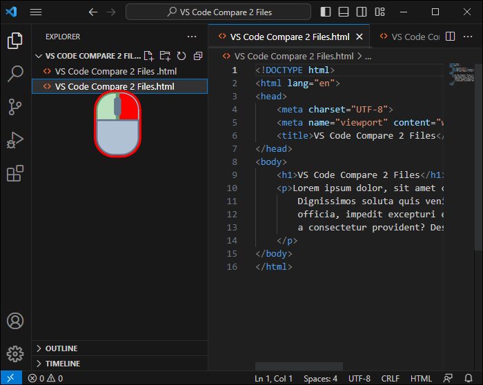
- Right-click on the tab of the first file that you want to compare.

- From the right-click menu that pops up, choose the option Select for Compare.
- Right-click on the tab of the second file you’d like to see on the right-hand side of the screen.
- Select Compare with Selected to view the differences.


Similarly, you can compare unsaved files and editors. Choose the first editor, click Select for Compare, and then Compare with Selected on the second editor.
Compare Different Git Versions
Comparing different Git repository versions is slightly different than comparing files on your own machine. You can do it this way:
- Go to the Explorer view.
- Select the file that you wish to explore through Git version history.
- Click on the timeline view to expand it and Click Git View File History.
- Click on the Git commit to see how it changed the file.


Compare Two Folders
You aren’t limited to only comparing files in VS Code. Here’s how you can compare the contents of two folders:
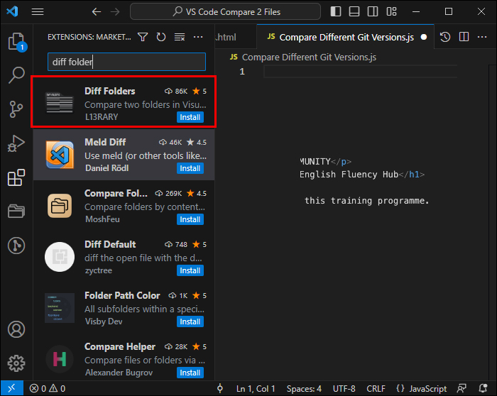
- Find and download the Diff Folders extension from the extensions console.
- Open the Diff folder view from your menu.
- Select the folders that you’d like to compare.
- Click Compare, and the contents will now show up.


Spotting the Differences
Once you pick two files for VS Code to compare, you will see the differences highlighted within your editor. That way, you can quickly tell what has changed in the code. Use the arrows in the toolbar to navigate through the changes. At this point, you can analyze the changes, debug, and determine which ones you’d like to keep or discard.
Merging Changes
If you have changes in one file that you’d like to incorporate into another, there’s an easy way to do it. All you need to do is find the merge icon on your toolbar and click it to merge the two files together.
Diff Viewer Explanation
Tucked away inside Visual Studio Code is a powerful difference viewer that lets users compare two versions of the same file or two entirely different files. This tool isn’t merely looking at something side-by-side — it makes it easy to tell what’s changed in the blink of an eye with convenient highlights.
When something has been removed from a file, it gets a bright red background on the left side and an angled pattern on the right. If there are additions in the second file (whether you choose the newer or older file as the second one), look for an angled pattern on the left and a bold green background on the right. When just parts of a line have been modified, they’ll get a light red and green background, so you don’t miss seeing where the changes happen to be. This way, you can quickly spot the differences and decide which changes you prefer.
Programming Language Aware Diff
Visual Studio Code’s diff viewer takes an effective line-by-line approach to compare files and highlight changed characters. This is a tried-and-true method that you might find familiar if you’ve ever used tools like Notepad++ and its comparison plugins. However, programming languages that allow for optional semicolons or line breaks can be problematic for this system as the diffs become quite noisy, with trivial edits littering the screen.
To combat this issue, there is an extension known as SemanticDiff, which looks beyond merely comparing text and parses the file’s code, assessing its compiler representation. This way, you can see past the small changes that don’t influence the program and instead directly identify moved code while providing a much clearer outlook on what matters in the diff. It’s akin to having a capable editor who understands the intricacies of coding language. It filters out the unimportant aspects and puts forth the adjustments that make a real difference once the code compiles.
If you want to gain more insight into code changes, install SemanticDiff from the VS Code marketplace and switch to smart diff mode to see the differences in your code with greater accuracy.
Find and Replace
Along with comparing, searching for specific text within a file or across multiple files is another task you will likely do frequently. VS Code’s find and replace functionality is robust with several advanced options:
- Press Ctrl+F to open the find widget in the editor to search within the current file. You can move through the results and even seed the search string from the selection.
- Run the find operation on the selected text by clicking the three-lines (hamburger) icon on the find widget or setting “editor.find.autoFindInSelection” to “always” or “multiline.”
- You can parse the text into the find input box to search multiple-line text. You can also resize the find widget.
- Press Ctrl+Shift+F to search over all files in the folder you currently have open. You can use advanced search options and glob pattern syntax.
- Match case, match whole word, regular expression, and case-preserving are some of the advanced options for finding and replacing.
Search Across Files
If you’re looking for something in particular across multiple files within the project, VS Code has got you. You can search quickly through all the files in the current folder with Ctrl+Shift+F. The results will be split into files that contain the query. You can also get creative and use regular expression searches to get more particular results.
Integrating File Comparison with Other Features
The power of diff tools within VS Code goes beyond file comparison. It opens up many integrated coding possibilities. By unifying features such as auto-save, Hot Exit, and advanced search, you can work seamlessly on one project while comparing different file versions and searching for specific functions across multiple files.
Furthermore, you can modify configuration files with absolute certainty that your changes will persist. You won’t have to worry about unsaved changes if the application is closed. Hot Exit remembers them all. All these features combined give you complete control of all your file versions and changes.
Compare With Care
Some coding tasks may seem more menial and tedious than others, and comparing two files is one such task. But VS Code’s diff tools and methods for comparing different data types make it easier and more pleasant. Easy-to-see highlights guide you through all the changes between two files and let you experiment with different code versions, all of which are excellent for debugging, analytics, and version control.
Do your projects call for tight version control and frequent file comparing? Do you have any tips or tricks regarding code-comparing methods? Share your thoughts and insights in the comments below.


Disclaimer: Some pages on this site may include an affiliate link. This does not effect our editorial in any way.