It’s an essential habit to factory reset your computer when you sell or dispose of it, regardless of whether it’s a Mac or Windows PC. It’s also best to factory reset it occasionally to remove all the bugs, unused data, and file corruption. Whether you use your PC daily for essential work or just the occasional picture viewing, resetting helps keep your system fast and efficient. Also, your device is bound to have all sorts of personal and sensitive information.
One of the best ways to wipe the hard disk clean, no matter the reason, is to reset your Windows PC, and if you’re running Windows 10, it’s relatively easy. Just be sure to back up your important documents, videos, game saves, images, licenses, and other essential data.
If you need to factory reset your laptop or PC and get it back to its original default settings, this article guides you through the reset process, and it works on any Windows 10 device.
Factory Reset Windows 10 using the ‘Reset Your PC’ Option
Before jumping into a factory reset of Windows 10, read this article in its entirety and check out the essential FAQs at the bottom. Afterward, you can decide if a factory reset is feasible.
It is important to note that the reset option may use the original OEM license if you upgraded your version of Windows 10, such as from Home to Pro. If that scenario applies to you, try to switch the license in the Settings menu.
If that process doesn’t work (most likely won’t), you must perform a clean install/upgrade using the newer license and software. Here are the steps to reset your Windows 10 device.
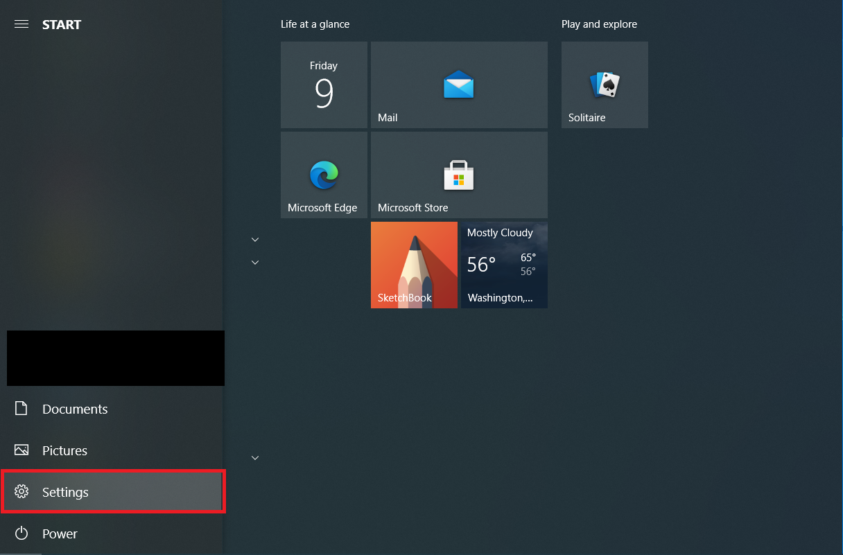
- Start by clicking on “Start Menu -> Settings.”

- Then, select “Update & Security.”

- From the “Update & Security” menu, select “Recovery” on the left side of the screen.

- Recovery will bring up a new page with additional options. For restoring your PC, you’ll want to select “Get started” in the “Reset this PC” section.

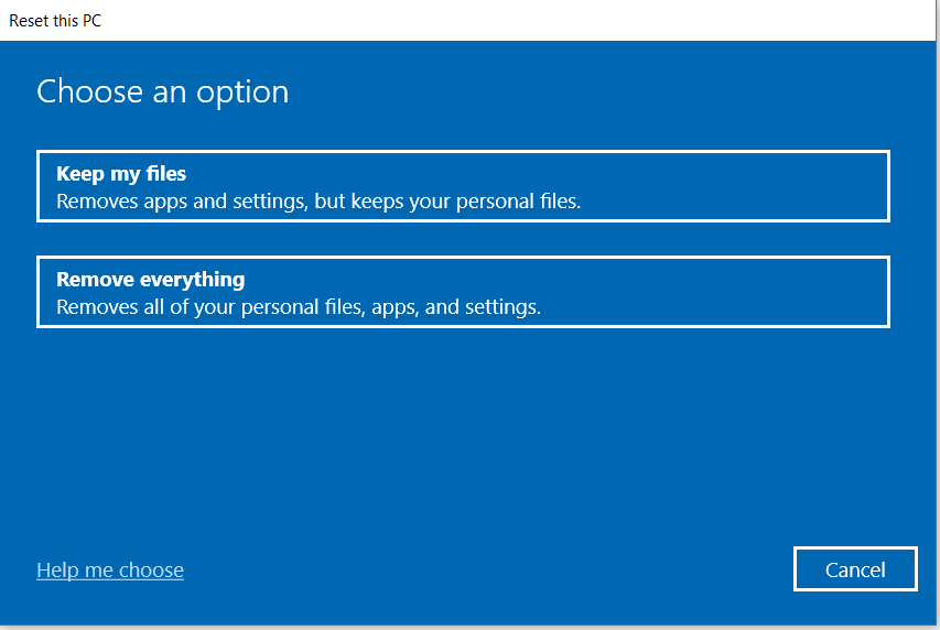
- Now, you’ll have two options: (1) “Keep my files“ or (2) “Remove everything.” The first choice will keep personal files and is suitable for generally refreshing settings and removing installed apps. The second choice will remove all files.

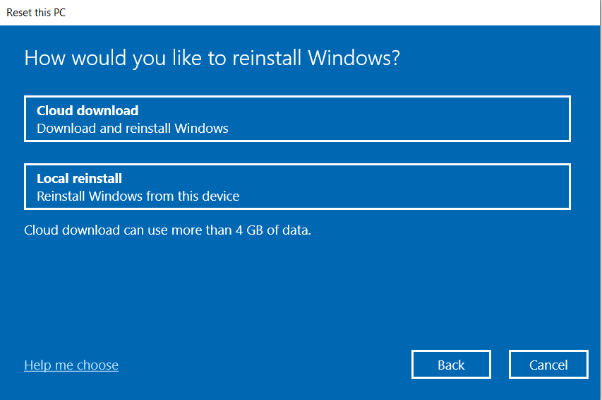
- If you use the “Keep my files” option above, you’ll see a new window. For Windows with the May 2020 Update or later, you’ll get two choices to reinstall Windows 10: “Cloud download” and “Local reinstall.” The cloud option reinstalls Windows 10 with the latest version. The local option uses existing installation data from your device.

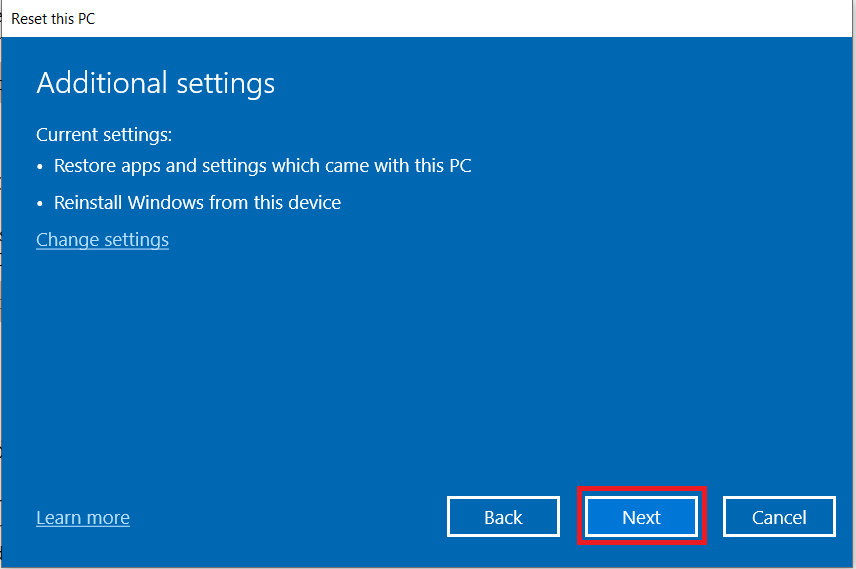
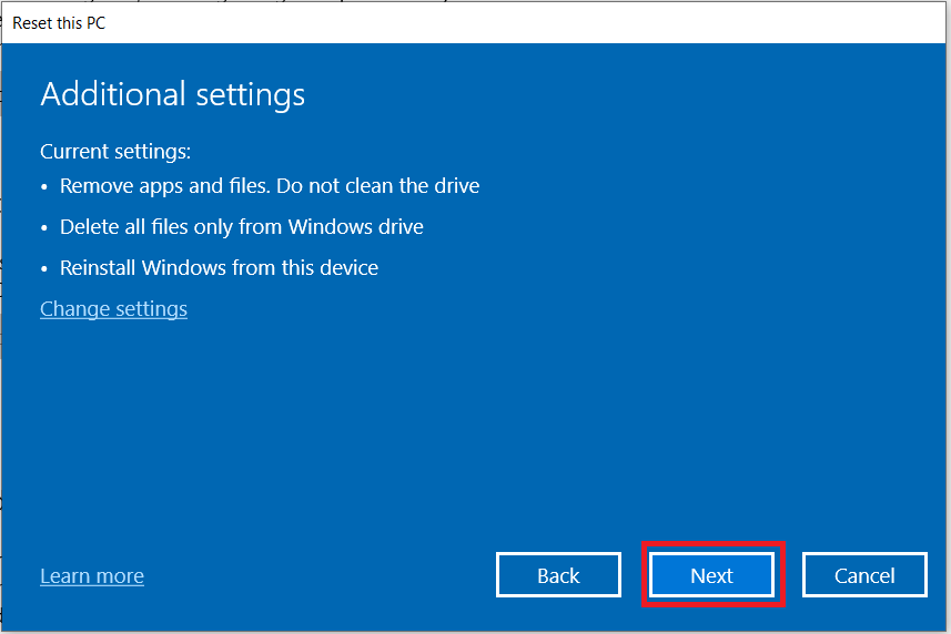
- You’ll now see the settings for what the reset will do. Click “Next” when ready.

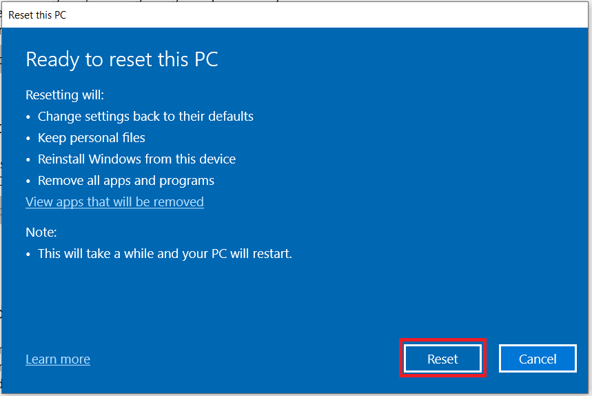
- Then, the “Ready…” screen will give you the option to view the list of apps that will be erased. Click “Reset” when ready.

- If you choose the “Remove everything” option, you’ll then need to select “Cloud download” or “Local reinstall” if you have Windows May 2020 Update or later.

- Next, you’ll be presented with the reset settings. Click “Next” when you’re ready.

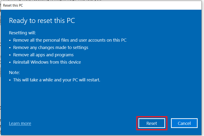
- Click on “Reset” in the next window to confirm your decision.

After the reset, you’ll see one or more HTML files on your Windows Desktop listing all deleted applications. You can decide what to reinstall from scratch.
Also, Windows 10 stores all old data in the “Windows.old” folder, so you always have the option to extract data from there if needed. Remember that most applications won’t have license information in Windows Explorer, but you can still search for valuable data.
Depending on your choices and your system’s speed, the reset will take up to an hour. You’ll know the process is finished when prompted with the license agreement.
If you’re not ready to reset yet but will be in the future, you can set Windows 10 to back up your files and automatically keep them updated between now and when you want to factory reset your laptop. However, the backup option is not for licenses and programs but for personally saved data. Some third-party backup programs offer independent file picking to restore installed/licensed programs.
Windows 10 Resets
As you’ve seen, there’s not much to resetting Windows 10. Ensure you have your important files backed up to a secure place before starting the process. Even if you keep files and reinstall the OS, it’s better to be safe than sorry.
Windows 10 Factory Reset FAQs
What’s the difference between a Windows 10 reset and a fresh start?
A Windows 10 reset is designed to reinstall the Windows 10 OS in its original OEM state when you purchased it. Therefore, all PREINSTALLED third-party applications and licenses that came with the device will get reinstalled. A Windows 10 fresh start is similar to a reset, except it DOES NOT preserve OEM and preinstalled third-party software and licenses—it reinstalls Windows 10 from scratch.
Note: Windows version 2004 (not a year) and up merged the “Fresh Start” option into the “Reset my PC” option.
Is it good practice to reset Windows 10?
Yes, it is a good idea to reset Windows 10 if possible, preferably every six months. Most users only resort to a Windows reset if they have PC problems. However, tons of data gets stored over time, some with your intervention but most without it.
The most commonly collected data includes your OS activities and your personal information. Actions like browsing history, social likes/shares, news views, search history, seen videos, document auto-saves, temporary backup files, bug reports, PDF view history, and more get stored on the system and used for specific purposes.
Data can accumulate quickly and rotate regularly, which slows your system down the more you use your PC. If left unattended, the data can be obtained from malware, spyware, and other means. Resetting your PC (like you might do with your Android smartphone) continually ensures optimum performance and stability. It also helps maintain privacy and security.
Does a Windows 10 reset save documents, music, images, and contacts?
Windows 10 preserves personal folders such as “My Documents,” “My Videos,” and “My Contacts” when performing a Windows 10 Reset. However, YOU MUST specify that you want to save that data when it prompts you. Otherwise, the reset will erase everything except OEM/preinstalled software and start from scratch.
Does resetting Windows 10 keep game data?
Typically, a Windows 10 reset DOES NOT save game data or games. The process is intended to provide a clean Windows OS, but it does offer an option to save some of your data, such as documents, images, etc. Independently installed or third-party installed games will not get backed up, but some now save to the cloud on their servers.
If you have games from the Microsoft Store, the saved data may get retrieved when you reinstall it, but that depends on the game’s functionality and options. Microsoft doesn’t personally handle saving files in the Microsoft Store.
Regardless, it is always best to back up any valuable game data before resetting your PC, and this will require research and unique methods based on the game saves and settings you need to preserve.
Does a Windows 10 reset save custom drivers?
No, a Windows 10 reset does not preserve any drivers. The OS reinstalls the default drivers or ones that Microsoft has in its database, so you’ll need to reinstall third-party or custom drivers yourself.
Does resetting my PC in Windows 10 require updates again?
Yes, a Windows 10 reset does not preserve updates, so you must reinstall them. However, the latest Featured Update includes all previous updates, so it won’t be so bad.
Disclaimer: Some pages on this site may include an affiliate link. This does not effect our editorial in any way.


