Although Windows 11 is supposed to be a more user-friendly operating system than its predecessors, it comes with a few surprising changes. Most notably, Microsoft has made it impossible to change the size of the taskbar through the Windows Settings. If you’re dissatisfied with the taskbar’s default appearance, you’re probably looking for a way to bypass the issue.
Fortunately, several methods will help you make the taskbar smaller. Keep reading to learn more.
How to Make the Taskbar Smaller in Windows 11
Making the Windows 11 taskbar smaller is relatively straightforward through the Registry Editor.
Before using this method, you’ll need to back up the editor to prevent compromising your device and data. To do so:
- Press Windows + R, type in regedit, and hit Enter to launch the editor. Alternatively, find it through the Windows search bar.

- Navigate to the upper left part of the editor and tap the Computer registry key. Once selected, the key will become highlighted.

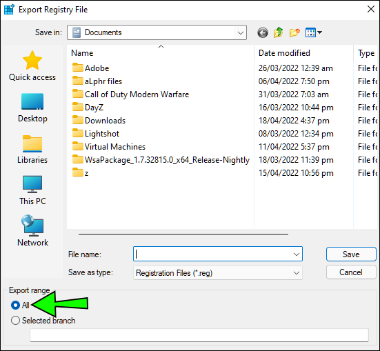
- Click on File and choose Export from the Editor menu. You can also right-click and press the Export option.
- The computer will generate a new window. Make sure that the All box is preselected.
- Select a new location to backup the files. It’s best to store them on the desktop or in the documents folder. Both are easily accessible when you want to use the editor to modify your system.
- Rename the file in the File name field.
- Click on the Save button. It typically takes the computer several seconds to complete the backup process.


Once the backup is stored in the selected location, you can change your system safely whenever you want to reverse the modifications using the backup files.
When you’ve backed up the registry data, you can resize your Windows 11 taskbar. Here’s how to do so manually:
- Hold Windows + R, type in regedit, and hit Enter or use the search bar to launch the Registry Editor.
- Now, go to
HKEY_CURRENT_USER\Software\Microsoft\Windows\CurrentVersion\Explorer\Advanced\by either typing/copying the path or manually navigating to it. - Hover the cursor over Advanced and right-click.
- Go to New > DWORD (32-bit) Value and click on it.
- The window will prompt you to enter a name. Type the following in the appropriate text field:
TaskbarSi. - Double-tap the TaskbarSi value to launch an editing box.
- To make the taskbar smaller, change the Value data to 0.
- Restart the PC to implement the changes.


Since the Registry Editor is one of the operative system’s most powerful programs, some users may feel uncertain about manually changing their system. Fortunately, it’s possible to resize the taskbar with a “.bat” file.
To modify the taskbar’s size with a downloaded file:
- Save the file to your local storage.
- Hover the cursor over the downloaded folder and right-click.
- Select the Extract All… option.
- Choose the location where you’ll store the extracted files and tap the Extract button.
- Open the unzipped folder and run the “.bat” file. Keep in mind that the file won’t resize the taskbar unless you run it as an administrator.
- When the Windows protected your PC alert appears, click on More info.
- Tap the Run anyway button, then sign in and out of your user account.


When you sign back in, the operating system will change the taskbar’s appearance and make it smaller.
Resizing the Windows 11 taskbar can also be done with a “reg” file. To do so:
- Download the files.
- Once the download is finished, unzip it to extract the files to a new location.
- Open the unzipped folder. It will contain three files:
- The “win11_taskbar_small.reg” file shrinks the taskbar.
- The “win11_taskbar_medium.reg” file returns the taskbar to its original size.
- The “win11_taskbar_large.reg” file makes the taskbar larger.
- Navigate to the win11_taskbar_small.reg file and double-tap it.
- Click on the Yes button to allow the file to change the computer’s system.
- A new window will notify you the file has finished modifying the system. Select OK to close the window.
- Reboot the PC and log in with your account information.


The taskbar will be smaller than usual when you power on the PC.
How to Restore Taskbar to Default Size in Windows 11
If you find that the smaller size isn’t working for you anymore, you might want to reverse the changes. Fortunately, Windows 11 allows users to enlarge the taskbar with the registry editor quickly.
- Tap Windows + R to launch the Registry Editor. If you prefer using the search menu, type
regeditin the text field and tap the Registry Editor option when it pops up. - Again, go to
HKEY_CURRENT_USER\Software\Microsoft\Windows\CurrentVersion\Explorer\Advanced\by either typing it in or manually navigating to the folder. - Place the cursor over the Advanced key and perform a right-click.
- Go to New > DWORD (32-bit) Value and click on it.
- When prompted to enter a name, type
TaskbarSiin the text box. - Double-click on TaskbarSi to edit it.
- Change the current Value data to 1.
- Reboot the computer to record the changes.


Another way of restoring the medium size is with a downloaded “reg” file, meaning you won’t have to change the data value manually. To use this method:
- Download the zipped files.
- Open the folder and save the files in a new location to unzip them.
- When you open the unzipped folder, you’ll find three options:
- The “win11_taskbar_small.reg” option makes the taskbar smaller.
- The “win11_taskbar_medium.reg” option restores the taskbar’s default appearance.
- The “win11_taskbar_large.reg” option enlarges the Windows 11 taskbar.
- Double-tap the win11_taskbar_medium.reg option and press the Yes button to permit the file to modify the PC’s system.
- A pop-up window will inform you that your system has been modified. Click on OK to close the notification.
- Restart the computer and log in with your account credentials.


When the operating system is up and running, you’ll see that your Windows 11 taskbar is back to its default size.
How to Make Taskbar Icons Smaller in Windows 11
There’s no direct way of resizing the taskbar icons on Windows 11 devices. The size of the icons is tied to the taskbar’s appearance. When the taskbar has a medium or default value, you’ll see medium-sized icons on your desktop. If you change the taskbar’s data value to “0”, tiny icons will appear over your screen. Finally, changing the data value to “2” enlarges the taskbar, so the computer will generate larger icons.
Users who think the taskbar icons are cluttering the lower end of the desktop may want to remove them and keep the screen tidy. To hide the taskbar:
- Hover the cursor over the taskbar, right-click on it, and select Taskbar settings.
- Click on the slider beneath Automatically hide the taskbar in desktop mode to enable the option.


When the mouse is away from the taskbar, it will disappear from the screen. Moving the cursor along the lower end of the desktop will bring up the taskbar.
FAQ
Can I remove the Task View icon from the Windows 11 taskbar?
Yes, it’s possible to remove the Task View icon from your taskbar. Here’s how:
1. Place the cursor over the taskbar, right-click, and select the Show the Task View button option.
2. Once you toggle off the button, the icon will be hidden.
Resize the Windows 11 Taskbar with Ease
Although the Windows 11 taskbar features a different appearance, it doesn’t have to spoil your user experience. We’ve covered several ways you can customize the taskbar and shrink it to match your personal preferences. If you feel it’s taking up too much space, you can hide it and declutter your desktop.
Have you resized your taskbar? Which of the above methods did you use? Let us know in the comments section below.


Disclaimer: Some pages on this site may include an affiliate link. This does not effect our editorial in any way.