Device Links
A good amount of video RAM is crucial for any visually-intensive PC game or task. If your computer has been struggling in this department lately, you might think upgrading your video card is the only solution.
While a new graphics card would undoubtedly boost your desktop computer’s visual performance, it’s not always an option for laptops. Video cards can also be rather pricey, so getting the most out of what you currently have can save you money for the time being. A solution that won’t require you to upgrade your hardware is increasing your PC’s dedicated video RAM. Read on to learn about this solution and how to implement it yourself.
Increasing Dedicated Video RAM
Video RAM (or VRAM) is RAM dedicated to the video part of a PC. Unlike regular RAM, VRAM works with your GPU to store short-term graphics-related data. VRAM is not the only factor determining how smooth your experience is while editing videos, rendering 3D models, or running graphics-intensive games. However, a certain amount of VRAM is necessary for these operations. While you can’t physically change your VRAM without changing your GPU, you can instruct your PC to use what you have to the fullest capacity.
Increasing your VRAM isn’t guaranteed to improve your experience, but it can help you bypass some obstacles. Try the following solutions on your Windows PC.
How to Increase Dedicated Video RAM in Windows 11
There are several ways to adjust VRAM in Windows 11, but you should also see what is currently being used before making any changes. Here’s how to check the current VRAM and the various options to change it.
Check the Currently Used VRAM Size in Windows 11
Before embarking on your journey to increase your dedicated video RAM, checking how much your Windows 11 PC currently uses is a good idea. Follow these steps to find that information.
- Click the “Windows” icon and go to your “Settings.”

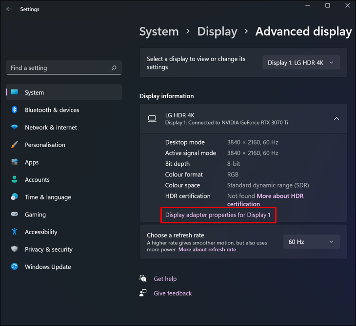
- Select the “System” settings menu on the far left, then choose “Advanced display” in the “Related settings” section on the right.

- Click “Display adapter properties for Display #.”
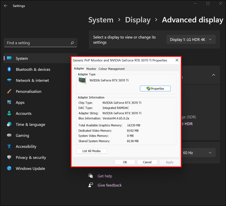
- You’ll see your dedicated video memory in the window that pops up.

Adjust Windows 11 VRAM Using the BIOS
If you find the amount of VRAM used in Windows 11 is insufficient, try adjusting it in your BIOS. Here’s how to do it.
- Restart your computer and repeatedly press your BIOS access button (F2, Del, etc.) while your PC boots up. Repeatedly pressing it ensures the action gets taken.
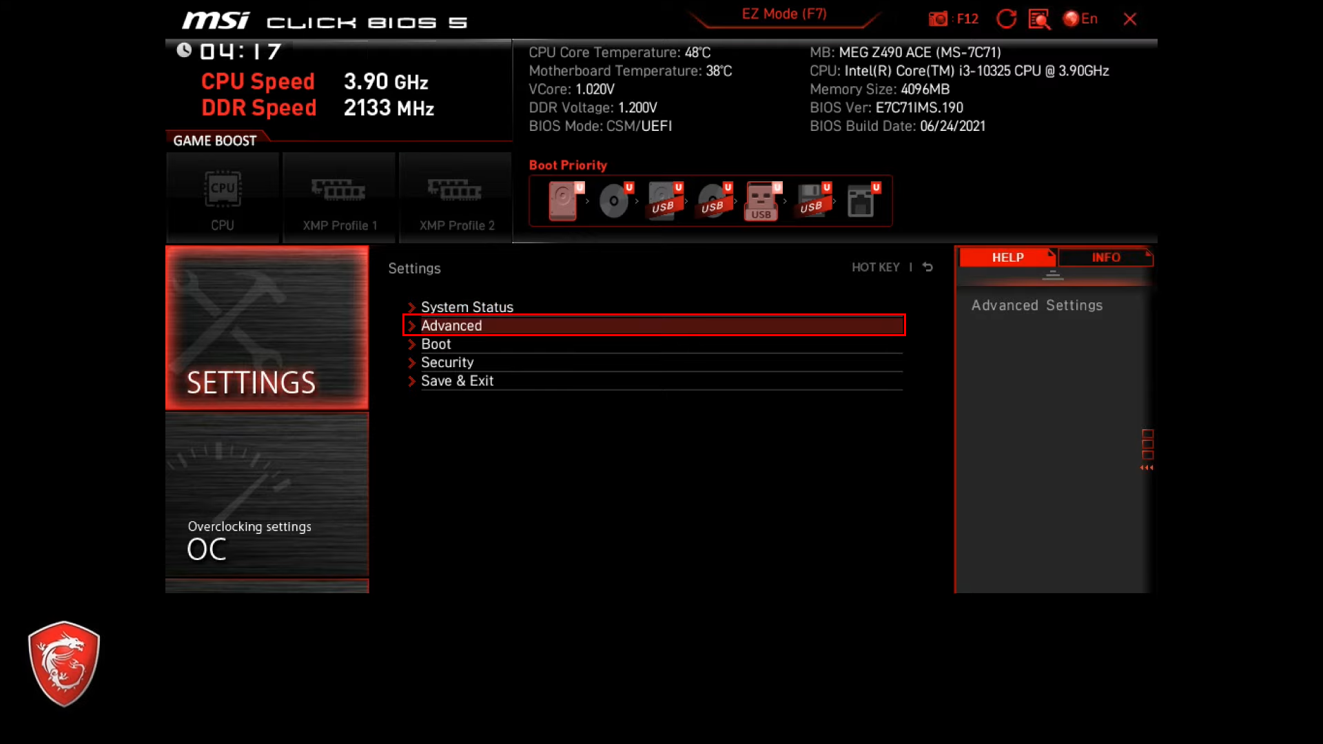
- Find the advanced features menu in your BIOS.
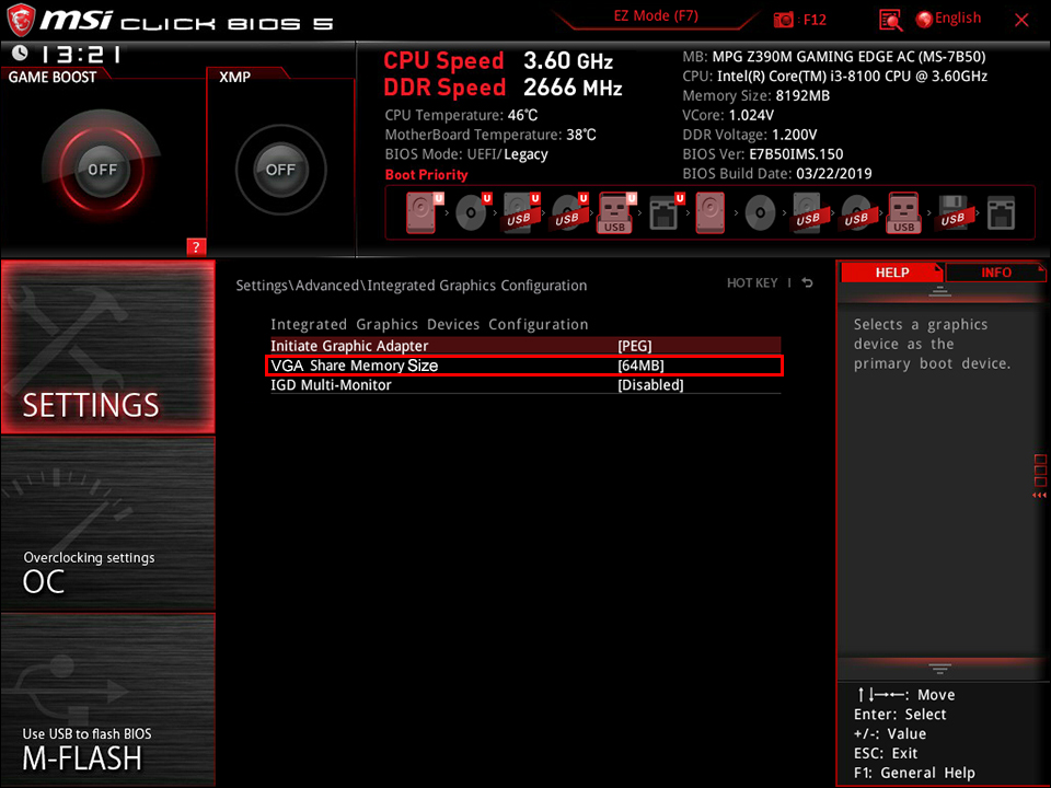
- Look for your VRAM graphics settings (the option to open may be labeled “Graphics Settings,” “VGA Share Memory Size,” “Video Settings,” or something similar).
- Choose the amount of space you want to allocate to your VRAM.
- Save the changes, restart your PC, and check whether your VRAM has increased using the abovementioned process.


Adjust Windows 11 VRAM Using the Registry Editor
Another way to tweak your dedicated Windows 11 video RAM is through the Registry Editor. While this won’t technically increase your VRAM, it will make programs believe they have more juice to work with.
Note that this trick may not work all the time. Some processes may exceed the actual VRAM limit if they are programmed to utilize/maximize what they use. In contrast, others set lower limits than what’s available, thus allowing them to use more since they believe more is available for use.
- Click your Windows icon, type “regedit” in the “search bar,” and open the “Registry Editor.”
- Navigate to the following location: “HKEY_LOCAL_MACHINE\Software\Intel.”
- Right-click “Intel” in the sidebar and select “New -> Key.”
- Name your new key “GMM” and open it.
- Right-click inside the right-side panel and select “New -> DWORD (32-bit) Value.”
- Name it “DedicatedSegmentSize” and double-click it.
- Select “Hexadecimal” on the right side and enter the amount of VRAM you want in megabytes.
- Click “OK” to save the changes, close the “Registry Editor,” then restart your computer.


How to Increase Dedicated Video RAM in Windows 10
The steps to increase your VRAM on Windows 10 are similar to Windows 11.
Check your current VRAM in Windows 10
- Type “advanced display” in the “Cortana search bar” and select “View advanced display info” to open the “Advanced Display Settings” window.
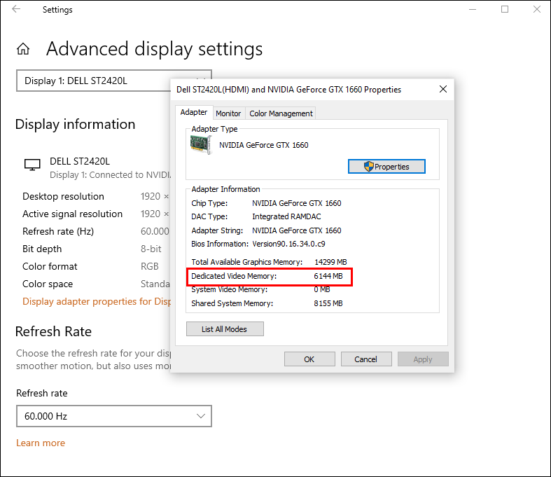
- Click “Display adapter properties for Display #” under “Display information.”
- Look at the number next to “Dedicated Video Memory” to determine your current amount of VRAM.

If the amount of VRAM is not to your liking, there are two ways to increase it without upgrading any hardware.
Increase VRAM in Windows 10 using the BIOS
- Restart your computer and repeatedly push your BIOS key (F2, Del, etc.) as the system boots up. Repeating ensures it accepts the keypress before booting up.
- Navigate to a menu called “Video Settings,” “Graphics Settings,” or “VGA Share Memory Size,” generally found in the “Advanced” menu.
- Increase the pre-allocated VRAM.
- Save the changes and restart your PC again.

Editing your BIOS isn’t an option for everyone. Fortunately, you can also tweak your VRAM using the Windows 10 Registry Editor.
Increase VRAM in Windows 10 Using the Registry Editor
While changing VRAM details in the registry doesn’t change the performance of your PC, it will trick programs that refuse to operate because of your currently low VRAM. Their performance may suffer, but they will at least run. More specifically, if a program limits what it allocates based on available VRAM, it will increase that amount and perform better. It could have issues if it assigns VRAM based on the maximum amount since you tricked it. This means that the process is experimental but often lets apps requiring higher VRAM to launch.
- Press “Windows + R” to open the “Run” dialogue box.
- Type “regedit” and hit “OK.”
- Navigate to “HKEY_LOCAL_MACHINE\Software\Intel.”
- Right-click “Intel” in the left-side panel and select “New -> Key.”
- Name the new key “GMM.”
- Right-click “GMM” and select “New -> DWORD (32-bit) Value.”
- Type “DedicatedSegmentSize.”
- Open “DedicatedSegmentSize,” select “Decimal,” and type a value between 0 and 512.
- Click “OK” and restart your PC to see the changes implemented.


How to Increase Dedicated Video RAM in Windows 7
For those still using Windows 7, increasing VRAM can be done using the Registry Editor, unlike Windows 10 and 11. Before you change the amount of dedicated VRAM on your Windows 7, verify your current VRAM in your Display Settings.
Check Your Current VRAM in Windows 7
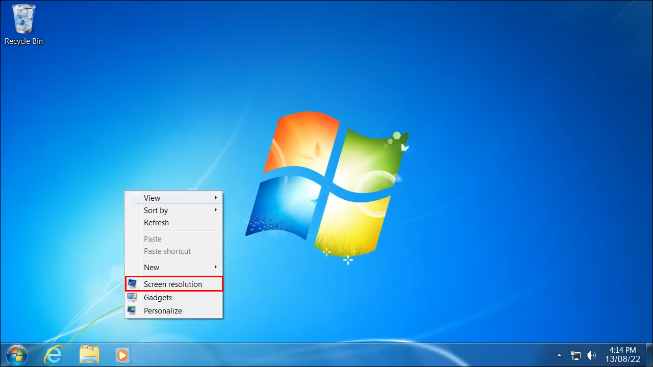
- Right-click on your desktop and select “Screen Resolution.”
- Find and select “Advanced Settings.”
- The currently allocated VRAM will be displayed next to “Dedicated Video Memory.”


Increase Windows 7 VRAM using the Registry Editor
To increase VRAM in Windows 7 to run software that requires a higher minimum to start up, follow these steps:
- Press “Ctrl + R” to open the “Run” window and type “regedit” followed by pressing “Enter” or clicking “OK.” You can also click the “Start Menu” icon, type “regedit” in the search box, and select “Registry Editor.”
- Click the “Edit” menu, then select “Find.”
- Type “INCREASEFIXEDSEGMENT” and click “Find Next.”
- Double-click the “IncreaseFixedSegment” file.
- Type “1” under “Value data” and press “OK.”
- Restart your PC and check your VRAM in your Display Settings using the first process above to see if your attempt was successful.


Overall, insufficient video RAM can easily lead to lags and freezes, which are annoying and can seriously hinder your work. If purchasing a new video card is not an option, you can try increasing your Windows 7/10/11 dedicated video RAM using the instructions above.
Related Posts

Disclaimer: Some pages on this site may include an affiliate link. This does not effect our editorial in any way.