The EA app is one of the best programs for installing and playing major Electronic Arts games. However, you may occasionally encounter error messages. One of the most common is the “Game is already running” pop-up window, which prevents you from playing the game on the platform. So, how do you fix it?
This issue typically appears due to corrupt cache data or interference from a similar application running in the background. Fortunately, troubleshooting this issue is relatively easy. Here are all the solutions to eliminate the “Game is already running” problem on the EA app.
How to Fix EA App Game Is Already Running Issue
Clear EA App’s Cache
Like any other application, the EA app stores cache data to offer faster service the next time you access the platform. However, sudden system shutdowns, malicious attacks, or viruses can corrupt the cache data. When this happens, you’ll likely encounter issues with the EA app, including the one at hand.
In this case, the solution is to clear the EA app’s cache data. Don’t worry; you won’t lose any data, although you’ll need to log in again with your credentials.
- In the top-left corner of the EA app, click the hamburger icon.

- Select Help.
- Choose App Recovery.

- Click Clear Cache.

The EA app will restart automatically; you must log in with your credentials. After logging in, check if you still face the issue. Restarting the app might also help fix the EA App keeps logging out issue.
Perform a Clean Boot
If closing a similar program that’s already running wasn’t helpful, the problem is likely caused by another service or program running in the background. You can identify the specific service or program by performing a clean boot. Here’s what you need to do:
- Open the Start menu, type msconfig in the search bar, and press Enter.
- In the System Configuration window, go to the Services tab.
- Select the checkbox for Hide all Microsoft services. Then, click Disable all.

- Go to the Startup tab and click Open Task Manager.
- Right-click on each startup program and choose Disable.

- Go back to the System Configuration window and click Apply and OK.
After that, restart your computer. Your computer will start in a clean boot state. Check if you still have a problem with the EA app. If not, then one of the programs you disabled was causing the issue.
To narrow down the specific program, follow the steps above again, but this time, select the checkbox next to one of the programs in the list to allow it to run when Windows starts up. If you don’t reencounter the problem, that program is not the culprit.
However, if the problem reoccurs after enabling the program, you’ve found the cause of the problem. You can disable it from running in the background if it’s a service. If it’s an application, you can try to uninstall it entirely if you no longer need it.
Reinstall the EA App
If none of the solutions work, your last resort is to reinstall the EA app. Here’s how to do it:
- Open the Start menu, type Control Panel in the search bar, and press Enter.
- Go to Programs.

- Select Uninstall a program.
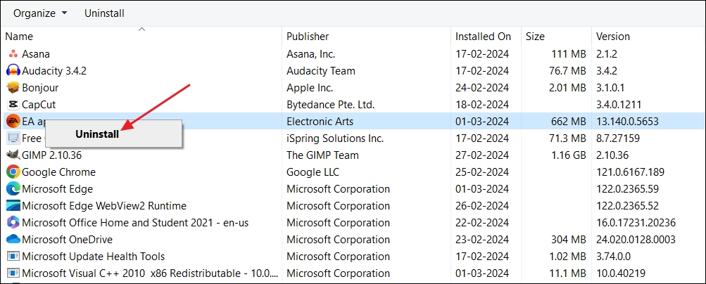
- Right-click on the EA app and click on Uninstall. Then, follow the on-screen instructions to complete the uninstall process.

Once you’ve uninstalled the EA app, head over to the official EA website and download the latest version.
Enhance Your EA App Gaming Experience
The issue of the “Game is already running” message is common for many EA app users. This can be quite a drag for gaming enthusiasts. Thankfully, there are ways to deal with it. The solutions listed above will help you eliminate the issue in no time. Once the EA app is up and running, you might want to learn how to change the language within the app.
FAQs
Suppose the EA app isn’t launching games. In that case, you can try solutions like running the EA app as administrator, temporarily disabling your antivirus or firewall, checking for software conflicts, and clearing the EA app’s cache data. If none of these work, you should reinstall the EA app.
Clearing the cache data deletes temporary files associated with the game saved by your computer. However, clearing the cache won’t affect your game data itself. Instead, it removes temporary files, which may cause some changes. For example, you might need to log in again and perform specific actions you wouldn’t have to do if the cache data wasn’t cleared.
Disclaimer: Some pages on this site may include an affiliate link. This does not effect our editorial in any way.


