Excel spreadsheets are a great way to store and analyze data, and they generally have cells with a combination of numbers and text. To understand your data more, you need to differentiate the cells with text. This process is a lot easier than it sounds.
This article explains how to select a cell range and then use the “COUNTIF” function to count the cells containing text. Let’s get started!
How to Count Cells with Text in Excel using Windows, Mac, or Linux
The process to count cells that contain text within your Excel spreadsheet on Excel 2007, 2010, 2013, 2016, 2019, 2021, and Excel 365 in Windows, Mac, or Linux is the same. Here’s how to do it.
- Click on any “empty cell” within your spreadsheet to insert the formula.

- Type or paste the function “
=COUNTIF (range, criteria)“ without quotes, which counts the number of cells containing text within a specific cell range.
- For “range,” enter the cell range you want to check. Type the first and last cells separated by a colon. For example, to count cells A2 to A9, you’d enter the following text string: “
A2:A9.” - For “criteria,” type
"*"with quotes. This part counts the number of cells that contain text within the specified range. The complete formula should look like the following: “=COUNTIF (A2:A9, “*”).” - Now, press “Enter” to apply the formula. The result will display in the formula’s cell.


How to Count Cells with Text in Excel on the iPhone App
To count the number of cells containing text within your spreadsheet using the Excel app on an iPhone, do the following:
- Launch the “iPhone Excel App.”
- Tap on “Open” to view your saved spreadsheets, then select the specific “Excel file” to open it.
- “Double-tap” on an “empty cell” in the spreadsheet to enter the “COUNTIF” formula, or you can “long-press” an “empty cell” and then tap “Edit” from the pop-up menu.
- In the empty cell, type in the following: “
=COUNTIF (range, criteria).” This formula counts the number of cells containing text inside your cell range. - For the “range” part, type the “cell range” you want to count. Enter the first and last cells separated by a colon. To calculate the number of cells within D2 to D12, type the following: “
D2:D12.” - For the “criteria,” type
“*”with quotes. This part counts the number of cells with text in the range. The complete formula should look something like the following: “=COUNTIF (D2:D12,“*”).” - Now, tap “Enter” to apply the created formula. The result appears in the formula’s cell.


How to Count Cells with Text in Excel on the Android App
To count the number of cells that have text in your spreadsheet using the Android Excel app, do the following:
- Launch the “Android Excel app.”
- The “Recent” menu opens by default. Tap on “Open” in the bottom-right section to open the “Places” menu, which is like a file browser.
- Browse and tap on the desired file to open it automatically.
- “Double-tap” on an “empty cell” to enter the “COUNTIF” formula. Alternatively, “long-press” any “empty cell,” then tap “Edit” from the pop-up menu.
- Enter the cell range you wish to count for the “range” part of the formula: “
=COUNTIF (range, criteria)” without quotes. This formula calculates the number of cells with text inside the cell range. - Enter the cell range you wish to count for the “range” part of the formula. Include the first and last cells separated by a colon. To calculate cells E2 to E12 from one column, enter the following text string: “
E2:E12.” - For the “criteria” part of the formula, type
“*”with quotes. This part of the text string counts the number of cells with text in the specified range, including more than one row. Your complete formula should look something like this: “=COUNTIF (A2:E12,“*”).” - Now tap “Enter” to apply the formula. The result appears in the formula’s cell.


How to Count Cells with Specific Text in Excel
By using the “COUNTIF” function, you can count the number of cells that contain specific text strings, such as “Excel,” “John,” or “John Meyers.” The formula is similar to counting cells with any text, but you change the formula’s “criteria” part to search for specific text. In this example, you’ll see the number of times the word “Excel” appears in a particular cell range:
- Click on an “empty cell” to type the formula.
- In the empty cell, type the following string without quotes: “
=COUNTIF (range, criteria).” - Enter the cell range you wish to count for the “range” part of the formula. Enter the first and last cells separated by a colon. To calculate cells A2 to A20, type the following string without quotes: “
A2:A20.” - For the “criteria” section of the formula, type
"Excel"with quotes. This part of the text string counts the number of cells with “Excel” in the specified range. Your completed text string should look like the following: “=COUNTIF (A2:A20, "Excel").”


How to Count Cells with Duplicate Text in Excel
Besides counting cells with text and specific text, you can count the number of cells with duplicate content.
In the following example, we’re looking for duplicate student grades.
- Column A – lists students (A2:A10)
- Column B – lists student’s grades (A, B, or C)
- Column D –lists available grades, including D2 for “A,” D3 for “B,” and D4 for “C.”
- Column E – lists the count of each grade.
Count Cells with Duplicate Text, Including First Instance
To count the number of cells in your spreadsheet with instances of grade “A,” “B,” or “C,” including the first instance, enter the following formula:
- For the grade letter “A,” click cell “E2” and type the following text string: “
=COUNTIF(B2:B10,D2).” - For instances of grade “B,” click cell “E3” and type the following text string: “
=COUNTIF(B2:B10,D3).” - For instances of grade “C,” click cell “E4” and type the following: “
=COUNTIF(B2:B10,D4).”


You now have the count for duplicate grades, including the first instance listed in column “E.”
How to Count Cells with Color Text in Excel
Excel does not have a specific formula to count cells based on their text color. To get around this, filter the results and then calculate the cells.
- Open the spreadsheet you wish to analyze.
- Right-click a cell with the text of the color you wish to count.
- Select “Filter,” then “Filter by Selected Cell’s Font Color” to filter the cells with the selected text color.
- Next, tell Excel to count your data range. If your text fills cells from B2 to B10, enter the following formula: “
=SUBTOTAL(B2:B10).”


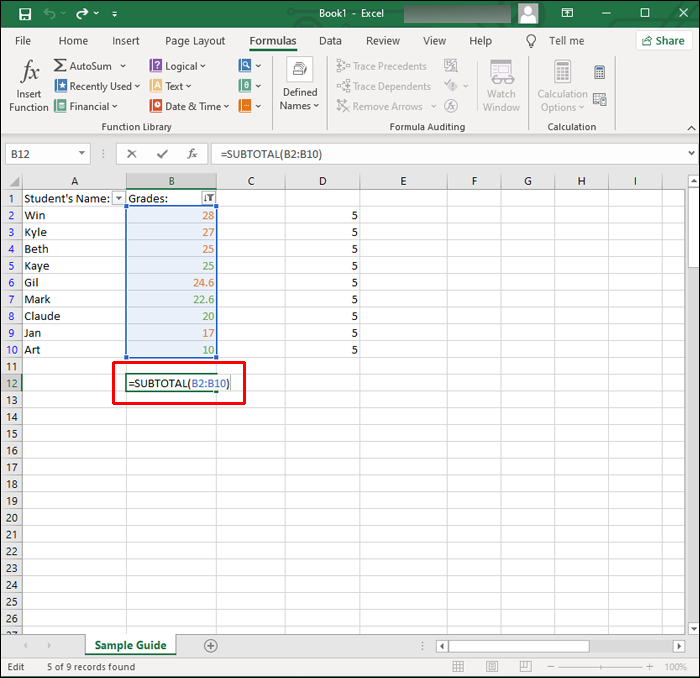
Once you hit “Enter” to apply the filter, Excel will only display the cells containing that color and hide the remaining values.
The “SUBTOTAL” function only returns the count for the selected text color and excludes the values in the hidden rows compared to “SUM.”
Wrapping Up
In closing, the Excel application does a great job of storing your data and facilitating analysis. It handles text as well as numbers. It has over four hundred functions, including “COUNTIF.” This function helps find the total of cells containing specific information, like cells with text, and the number of occurrences for particular text strings whenever you need to sort through a bunch of data to find what you need.


Disclaimer: Some pages on this site may include an affiliate link. This does not effect our editorial in any way.