How To Merge Tabs in Excel

Excel is an incredibly useful tool for storing, managing, and displaying large sets of data. Whether you’re handling repeatable results of scientific experiments, company employee information, surveys of product prices, or more, these all can be displayed as spreadsheets in Excel.

An Excel file, or workbook, may contain multiple tabs. While most Excel sheets have different uses, some tabs might contain duplicated or related information. Merging, or consolidating, related tabs into a single Excel tab will help you read, analyze, and organize the data for further processing.

This article will show how to merge two (or more) tabs in Excel, along with some advanced features and methods you can use.

Merging Tabs in Excel – It’s Simple

Before merging, make sure all tabs have backup copies. Your source tabs will contain the raw data you’re using, while the destination tab will have the final result. Depending on your project requirements, these may or may not be the same tab.

The default consolidation function in Excel can merge data by position or by category (row or column name). However, the data needs to be in the same format and size, or it will create new rows or columns. For example, if you’re using sales metrics for different offices, you need to have the same number of categories you’re sorting by, and the same number of weeks/months you’re cataloging.

Keep in mind that the consolidation functions work with numeric data. Excel can calculate sums, averages, deviations, and minimum and maximum values, among other statistical points. However, it doesn’t allow for more nuanced transformations of text-based data.

The steps for merging, by position or category are shown below:

1. On the destination tab, decide the positions for the merged data and click the upper-left cell of the selected positions.
   
   
   
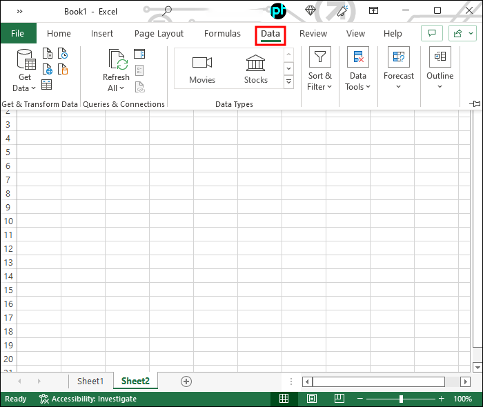
2. Click on the “Data” tab.
   
   
   
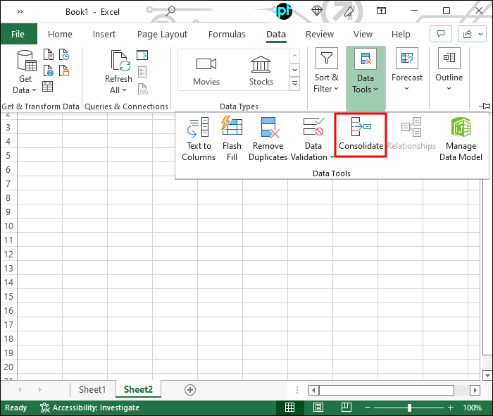
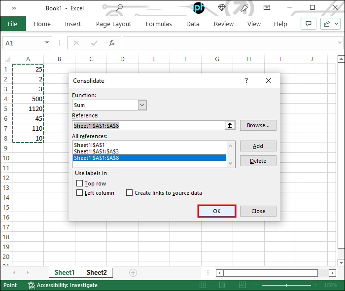
3. Go to “Data Tools” and select “Consolidate.” This opens a pop-up window.
   
   
   
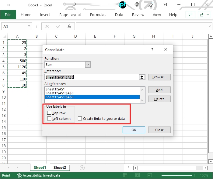
4. In the “Function” box, select a function from the dropdown list.
   
   
   
5. Select the data to be merged:
   
   • If by position, go to “Source Tabs” and click the “Add” button to add the data into the “All references” box. The data to be added can be manually typed in, such as “Sheet1!$B$2:$B$10” refers to the cells from B2 to B10 of the tab named Sheet1 in the current document.
     
     
   • If by category, in the “User labels in” box, select “Top row” (by rows) or “Left column” (by columns), or “Create links to source data” (write in links).
     
     
     
6. Click the “OK” button, and the data in the “All References” box or selected rows/columns will be merged.
   
   
   

It should be mentioned that you can always use copy-and-paste to transfer data from one tab to the other. However, this can be time-consuming and prone to errors. There are more elegant ways to achieve consolidation without repeating information.

Merging Tabs in Excel VBA

VBA stands for Visual Basic for Applications, a simple yet powerful programming language you can use to extend Microsoft Office applications, including Excel. The main issue in using VBA is that you will need to understand and use code to create applications or macros.

To create and edit a VBA Macro, do the following:

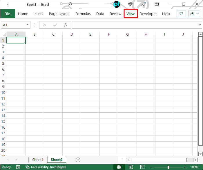
1. Select “View” in the toolbar.
   
   
   
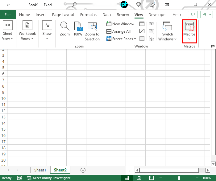
2. Click on “Macros” on the far right. This opens a pop-up Macro window.
   
   
   
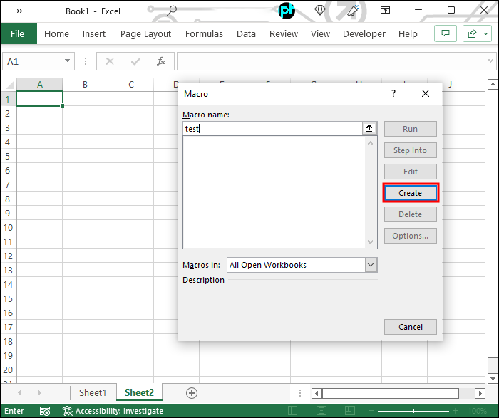
3. Type in the macro name (for example, “test”) and click the “Create” button at the right side and a coding console will pop up with the basic contents which read something along the lines of:
   
   ###
Sub test()
End Sub
###
   
   
   
4. You can edit the Macro code in the console. This is an example that combines tables from sheets:
   
   ###
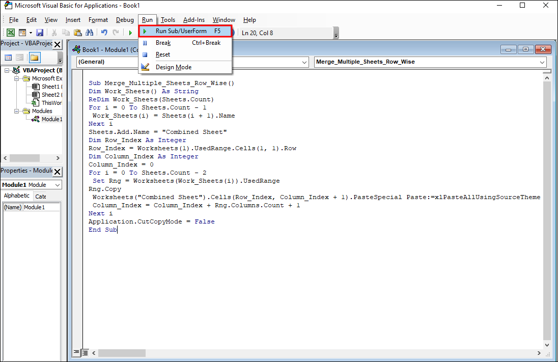
Sub Merge_Multiple_Sheets_Row_Wise()
Dim Work_Sheets() As String
ReDim Work_Sheets(Sheets.Count)
For i = 0 To Sheets.Count - 1
 Work_Sheets(i) = Sheets(i + 1).Name
Next i
Sheets.Add.Name = "Combined Sheet"
Dim Row_Index As Integer
Row_Index = Worksheets(1).UsedRange.Cells(1, 1).Row
Dim Column_Index As Integer
Column_Index = 0
For i = 0 To Sheets.Count - 2
 Set Rng = Worksheets(Work_Sheets(i)).UsedRange
Rng.Copy
 Worksheets("Combined Sheet").Cells(Row_Index, Column_Index + 1).PasteSpecial Paste:=xlPasteAllUsingSourceTheme
 Column_Index = Column_Index + Rng.Columns.Count + 1
Next i
Application.CutCopyMode = False
End Sub
###
   
   The sample macro code loops over the total number of Tabs and creates a new sheet “Combined Sheet.”
   
   
   
5. To run the code, in the Macro console, in “Run” tab, click “Run Sub/UserForm”, then the new Tab named “Combined Sheet” will be generated. You can also modify the Marco code to edit the data range and names.
   
   

Merging Sheets in Excel Online

Multiple free online tools allow you to merge Excel sheets. In these tools, you simply need to select and upload the workbooks (either a muti-Tab workbook or different workbooks). Examples are Aspose Cell Merger and DocSoSo Excel Combiner.

Keep in mind that merging sheets doesn’t manipulate the data. These tools take two or more Excel workbooks and return an Excel workbook with one or more sheets with data copied into them.

Combining Tabs in Excel Using Power Query

Power Query is another way to combine Tabs in Excel. For an Excel workbook with multiple tabs, use the following steps:

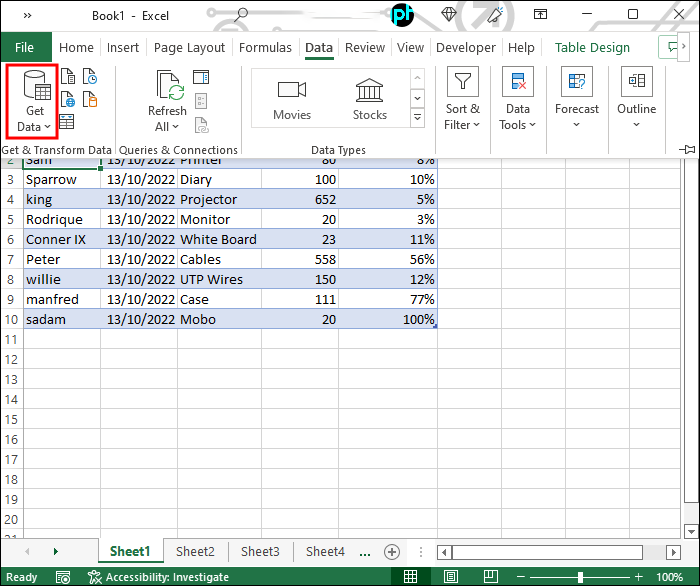
1. Go to the “Data” tab and the “Get & Transform Data” group, and click on the “Get Data” button.
   
   
   
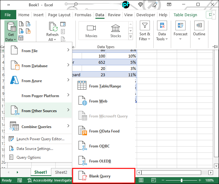
2. From the list, click “Blank Query” in the “From Other Sources” option, and you will see a new Power Query Editor with the default name “Query 1.”
   
   
   
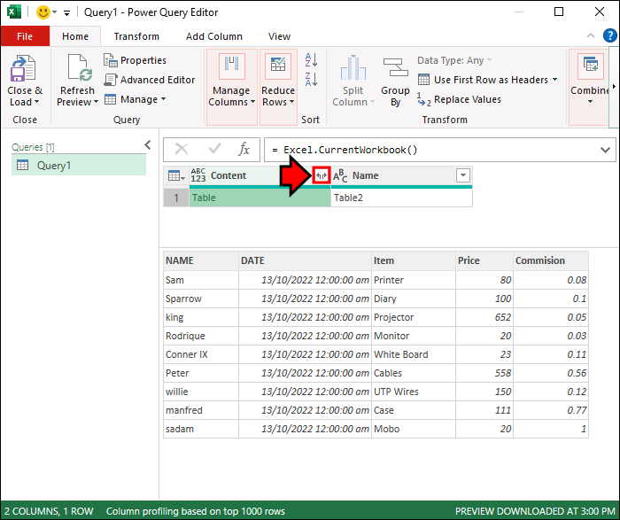
3. In the function (fx) bar, type the formula “=Excel.CurrentWorkbook()” (note the formula is case sensitive), and hit the “Enter” key and a list of the Tab names of the original workbook will appear.
   
   
   
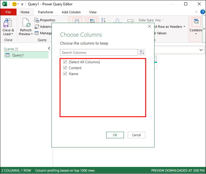
4. Select the tab names (columns) for merging (or mark the option “Select All Columns” if all columns are to be merged).
   
   
   
5. Click the double-arrowed button nearby the “Content” key.
   
   
   
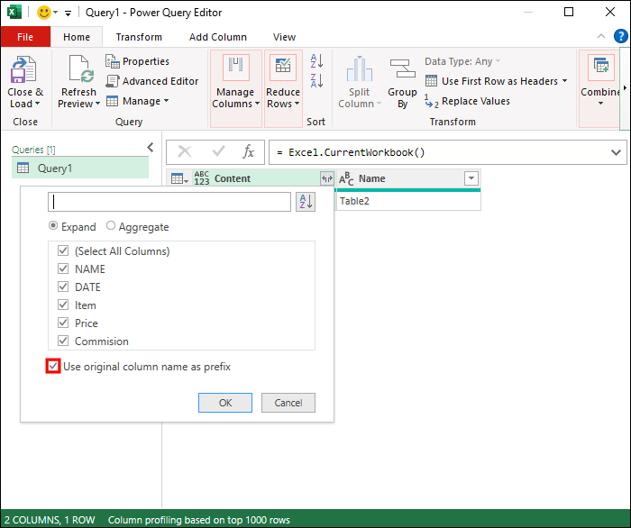
6. Unmark the “Use original column name as prefix” if you want the exact names in the original workbook to be used in the merged file instead of as prefixes.
   
   
   
7. Click “OK” and you will see a new tab with all merged data, in which the tab names of the original workbook will be listed in the right-most column.
   
   

Alternative Methods

Excel is a useful tool for handling 2D array data. If you are a data scientist, however, you may access the data directly using programming languages such as Python or R. The key is that the data structure of the 2D arrays is common: using separators (space, tab, comma, etc.) to split all data points. The .csv format, for example, uses comma separators and can be directly opened for reading/editing by Microsoft Excel. Alternatively, you can also open the Excel files (.xlsx) by these programming languages, such as the “readxl” package in R, which can open and handle the data from different Excel worksheets. In these cases, simple yet convenient functions, such as cbind (binding columns with the same dimension) can be used for merging. All data from different Excel Tabs can be merged into data frames for statistical analyses and visualizations, without using the Microsoft Excel software.

Get More Out of Less

From the processes summarized above, you will get a single integrated worksheet with data from multiple resources. This worksheet can serve as an archive or backup database. Moreover, the merged tab allows you to acquire perspectives that may be missing from the data from a single resource. We encourage you to test the consolidation functions and macros on example data and back it up beforehand.

Do you have a better way to consolidate tabs in Excel? Let us know in the comments below.

Related Posts

How To Merge Tabs in Google Sheets How to Merge PowerPoint Files into a Single File How To Merge Two Faces Easily with Several Different Tools How to Open the Merge Editor in VS Code How to Revert a Merge in Git How To Make Text Fit in a Cell in Excel